Statistics I: General Description

Statistical tools are grouped according to function. Some tools serve to describe a large group of information in just a few numbers. These tools are called “descriptive statistics.” Other tools tools test to see whether the information obtained is close to what should be expected. These tools are called “inductive statistics.” They have that name because they are based on inductive logic: key terms in the formulas are derived from observation rather than deduced from a definition. In this unit, we will consider descriptive statistics (average and standard deviation) and two inductive statistics (Student’s t-test and Chi-square). The next unit (Statistics II) will be devoted to the most commonly used inductive statistics—correlation and analysis of variance.

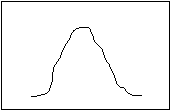
“Distribution” is the statistician’s name for all of the observations you have made about a single characteristic (like the number of people per household, the age of the people in the region, or the number of people using a department’s services each day last month). If all the observations for any of these characteristics were ranked from highest to lowest, and then plotted on a graph, it might look like this:

Normal Distribution

What you see is a “number line” along the bottom (the “X” axis), and the number of observations counted along the side (the “Y” axis). The graph shows that at the beginning and the end of the observation cycle, a relatively few people used the department’s services; rising to a peak in the middle of the observation period..

Descriptive statistics are designed to express the same information displayed in Figure 1, only to do it with a few mathematical expressions. Charts are useful because they can present a large amount of information (“data”; one item from the data is called a “datum”) in a fairly compact form that is often easy to grasp, at least in its broad outlines. On the other hand, the information from charts cannot be directly inserted into other mathematical statements, nor do charts lend themselves to a precise summary. That is what descriptive statistics are for.

The most common descriptive statistics are the three “measures of central tendency”: mean (or average), median, and mode. The mode is the measurement category that occurs most frequently (in Figure 1, it is right in the middle). The median is the observation that falls exactly in the middle of the distribution, when the observations are ranked from lowest to highest (in Figure 1, is also right in the middle). The means is the “weighted center” of the observations; if the number line were thought of as a balance, the mean would be the point where the line balanced (in Figure 1, it is again in the middle).

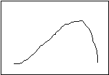
You have, no doubt, noticed that the three measures returned the same result in the example. This is not always the case; if it were, there would be no need for three different measures. The first example I gave you was a nicely balanced distribution. Such things are rare in the real world. Usually, the distribution is skewed to one side or the other, as in the following figures:

Positive Skew Negative Skew

In a positively skewed distribution, the median (the exact middle of the observations) is pulled to the right (the “positive” direction) of the mode (the most common distribution), and the median (the “balance point”) is pulled even more to the right. In a negatively skewed distribution, the arrangement is reversed—the mean and the median are pulled to the left (the “negative” direction). Notice, then, that the relative location of the three measures of central tendency can tell you if a distribution is skewed, and in which direction.

Since there are three measures, how do you decide which one to use? If the distribution is fairly balanced (each side is a reflection of the other), the three measures are roughly comparable. There are many other statistical tools, however, which use the mean (or other measures based on the mean) as part of the calculations. For that reason, the mean is the preferred measure of central tendency. However, if the distribution is badly skewed, the mean will not be a useful measure since it is affected most by imbalance. In those cases, the median is most commonly reported. Income, for example, is usually a skewed distribution; it is customary to report the median personal or household income rather than the average.

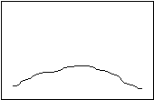
In addition to the measures of central tendency, descriptive statistics also include measures of dispersion. Two distributions can have the same mean, yet look very different, as in the following:

Platykurtosis Leptokurtosis

Although both distributions might have the same mean, the first one shows relatively similarly values all along the distribution, while in the second one the observations are lumped together near the mean. “Kurtosis” is a Greek word that means “curved.” “Platy” means flat, and “lepto” means “thin.” Standard deviation, the most common measure of dispersion, is a measure of the average (or “standard”) deviation of each datum from the mean. The larger the standard deviation, the more spread out the data. If two distributions have the same standard deviation, their general outline must be the same. There may still be some minor variation, but it will be slight. In this chapter, you will learn how to calculate the mean and the standard deviation.

In this unit you will also learn two inductive statistics, one parametric (Student’s t-Test) and one nonparametric (Chi-square). The difference between them lies in the assumptions you can make about the “true” distribution of the data. All inductive statistics work from observed data to create an estimate of the “true” or “population” distribution. Rarely will you have the luxury of actually observing the totality of the phenomenon you are interested in; most of the time, you must settle for looking at a representative sample of the data.

Parametric statistics assume that the true distribution is “normally” distributed. The “normal” distribution is the name given to the way things distribute themselves when they are independent of each other. The sands in an hourglass come to rest in a “normal” distribution. If a test is well-constructed, scores on the test will fall into a “normal” distribution.

Nonparametric statistics make no assumptions about the shape of the underlying distribution. Since they make fewer assumptions (they still assume the rules of probability), they can be used in more instances. There is a price to pay for the increased flexibility, however. Nonparametric statistics are also less sensitive. They are more likely than parametric statistics to overlook a small, but still significant, difference in the data. Chi-square tests whether the observed interaction between two variables could be obtained by chance from a larger population, just from knowing how many in the sample belong in the various categories of each of the variables.

The simplest of the parametric statistics compares an observed distribution to an ideal distribution or to another observed distribution, and tests for the fit between them. “Student’s t-Test,” a statistic you will learn in this unit, is one such tool. Since observation is based on only a sample of the entire population of events or traits, it is likely that samples drawn at different times will return slightly different observations. So it is important to know whether observed differences are small enough that they could just be due to sampling “error” (or variation), or whether the differences are large enough tojustify the claim that there is a “significant” difference. In the next unit, you will learn other, even more powerful parametric statistics.

Next Section

Back to Syllabus

609