Calculating a Linear Program
The process
for calculating a linear program is fairly straightforward: Specify the constraints as inequalities
(formulas), and solve them simultaneously (substitute one into the other to
find their common solution, or—alternatively—plot the equations on a common
graph to find their intersection). The
trick, of course is to convert the information at hand into formulas that will
be useful.
Consider
an example:
1.
Suppose a city
department has 54 employees—36 office staff and 18 field workers. The department has 2 functions, planning and
maintenance, each of which requires some effort from both groups. The labor requirements are as follows:
|
|
Maintenance (x) |
Planning (y) |
|
Office |
1 |
2 |
|
Field |
1 |
.5 |
2.
And, since
production cannot be negative,
a. Maintenance > 0
b. Planning > 0
3.
Ideally, how
much should the department provide of each service?
Therefore,
·
From 1,
office labor requirements are x
+ 2y > 36
·
From 1, field
labor requirements are x
+ .5y > 18
To solve a
family of equations, you need as many equations as you have unknowns. Converting the first two to equalities, and
substituting:
x + 2y = 36, so y = 18 - .5x
x + .5y = 18, so x + .5 (18 - .5x) = 18 so
x + 9 - .25x = 18
so x =
.75 (9) = 12
and 12 + 2y = 36, so y = (36 – 12) / 2 = 12
Returning
these values into the formulas, we find that the ideal distribution of office
labor will be 12 in maintenance and 24 in planning; field labor will be 12 in
maintenance and 6 in planning.
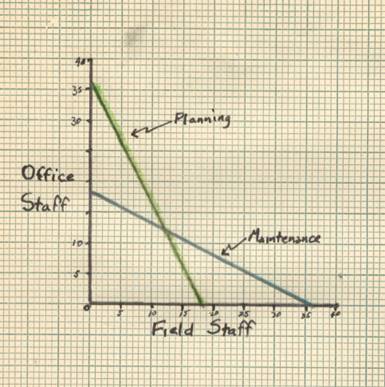
The
same result could have been obtained graphically:
© 1996 A.J.Filipovitch
Revised 11 March 2005